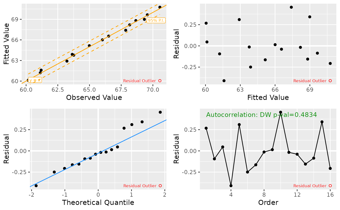
Generates a 4-panel diagnostic plot for a multiple regression model, including: 1) Fitted values vs. observed values (check for non-linearity), 2) Quantile–Quantile plot of residuals (check for non-normality), 3) Residuals vs. fitted values (check for heteroskedasticity), 4) Autocorrelation for time series otherwise influence plot (leverage also available).
Arguments
- mdl
A fitted model object (typically from
lm).- ...
Additional arguments (not currently used).
- is.ts
Logical;
TRUEif data are time series,FALSEotherwise.- pred.intvl
Logical; plot prediction interval on fitted vs observed.
- pval.SW
Logical; include Shapiro–Wilk p-value in
qqplot.- pval.BP
Logical; include Breusch–Pagan p-value in
varplot.- pval.DW
Logical; include Durbin–Watson p-value in
acplot.- cook.loess
Logical; overlay Cook's distance loess curve in
inflplot.- rtn.all
Logical; return all plots and parameters (vs. 4-way plot only).
- plt.nms
Character vector of which panels to plot. Defaults to fit, var, qq, and ac/infl depending on
is.ts(Order: start upper left, continue clockwise)- parms
List of overrides to plot formatting parameters (see
lm_plot.parms).
Value
A ggplot object representing the 4-way diagnostic panel.
Optionally invisibly returns a list containing:
p_4way– the combined plot,other elements passed through from the individual plot functions.
Details
This function is a high-level wrapper that calls internal plotting functions
(lm_plot.fit, lm_plot.var, lm_plot.qq, and either lm_plot.ac or
lm_plot.infl) and assembles their outputs into a combined plot_grid.