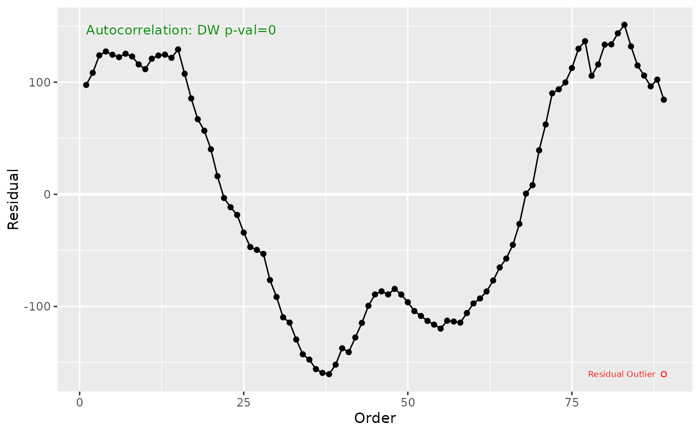
Creates a plot of residuals against the sequence/order of observations to visually assess independence and detect autocorrelation. Outliers are labeled by default. Optionally includes p-value result from the Durbin–Watson test for autocorrelation.
Usage
lm_plot.ac(
  mdl,
  ...,
  pval.DW = FALSE,
  parms = lm_plot.parms(mdl),
  df = lm_plot.df(mdl, parms = parms)
)
Arguments
- mdl
A fitted model object (typically from
lm).- ...
Additional arguments (not currently used).
- pval.DW
(logical, default = FALSE) Option to show Durbin-Watson p-value on the plot.
- parms
A list of plotting parameters, usually from
lm_plot.parms().- df
Data frame with augmented model data. Defaults to
lm_plot.df(mdl).
Value
A ggplot object representing the residuals vs. order plot. Included as an attribute "parm" is a list containing:
limPlotted limits onxandyaxes,pval.DWOption to show Durbin-Watson p-value,DWThehtestobject with Durbin-Watson test results.
Details
Points are colored and shaped according to whether they are residual outliers
(as determined by Tukey's boxplot rule). The function can label points using
ggrepel if parm$pts$id$outl or parm$pts$id$reg are set to TRUE.
Examples
fit <- lm(res ~ ., data = data.frame(time = time(austres), res = austres))
lm_plot.ac(fit, pval.DW = TRUE)