Plot Observed vs. Fitted Values to Check Linearity

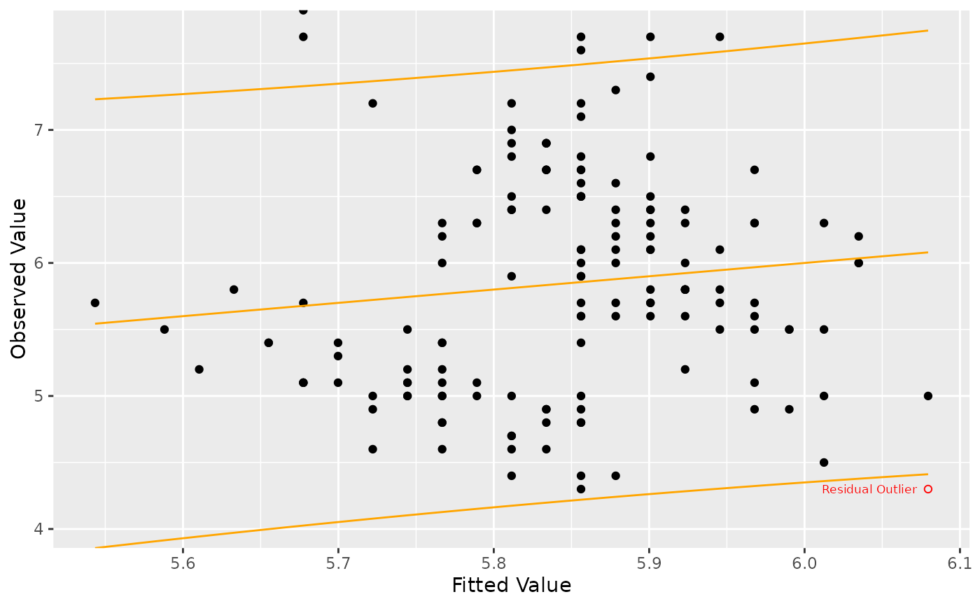
Generates a scatter plot of fitted values versus observed values from a linear model, with identification of outlier points and optional prediction interval. The plot includes a reference line y = x for assessing linearity.

Usage

lm_plot.fit(
  mdl,
  ...,
  pred.intvl = TRUE,
  parms = lm_plot.parms(mdl),
  df = lm_plot.df(mdl, parms = parms)
)

Arguments

mdl

A fitted model object (typically from lm).

...

Additional arguments (not currently used).

pred.intvl

(logical, default = TRUE) Option to show prediction interval bounds of fitted values.

parms

List of plotting parameters, usually from lm_plot.parms().

df

Data frame with augmented model data. Defaults to lm_plot.df(mdl).

Value

A ggplot object representing the fitted vs. observed plot. Included as an attribute "parm" is a list containing:

• lim Plotted limits on x and y axes,

• pred.intvl Option to show prediction interval,

Details

The plot visualizes fitted versus observed values, includes a diagonal reference line, marks outliers, and can optionally display prediction intervals. Outlier and regular points can be labeled. This plot is useful for visually assessing linearity and model fit quality.

See also

lm_plot.df, lm_plot.parms

Examples

mdl <- lm(Sepal.Length ~ Sepal.Width, data = iris)
lm_plot.fit(mdl)