Q-Q Plot of Residuals to Assess Normality

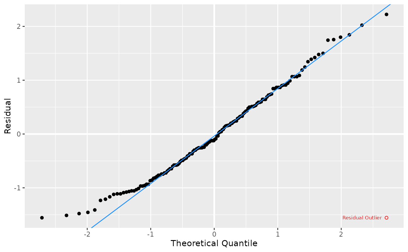
Produces a Q-Q plot of residuals from a linear model to test for normality, optionally annotating outlier points and adding the Shapiro-Wilk test p-value.

Usage

lm_plot.qq(
  mdl,
  ...,
  pval.SW = FALSE,
  parms = lm_plot.parms(mdl),
  df = lm_plot.df(mdl, parms = parms)
)

Arguments

mdl

A fitted model object (typically from lm).

...

Additional arguments (not currently used).

pval.SW

(logical, default = FALSE) indicates whether to include Shapiro-Wilk p-value on the plot.

parms

List of plotting parameters, usually from lm_plot.parms().

df

Data frame with augmented model data. Defaults to lm_plot.df(mdl).

Value

A ggplot object representing the quantile-quantile plot. Included as an attribute "parm" is a list containing:

• lim Plotted limits on x and y axes,

• pval.SW Option to show Shapiro-Wilk p-value,

• DW The htest object with Shapiro-Wilk test results.

Details

The plot visualizes the distribution of residuals against theoretical normal quantiles. Points are colored and shaped by outlier status, and a reference Q-Q line is added. Optionally, outlier and regular points can be labeled. If enabled, the Shapiro-Wilk normality test p-value is displayed.

See also

lm_plot.df, lm_plot.parms, shapiro.test

Examples

mdl <- lm(Sepal.Length ~ Sepal.Width, data = iris)
lm_plot.qq(mdl)