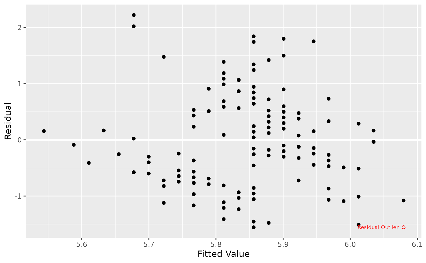
Produces a scatter plot of residuals against fitted values from a linear model, highlighting outlier points and optionally displaying the Breusch-Pagan test p-value for heteroskedasticity.
Usage
lm_plot.var(
  mdl,
  ...,
  pval.BP = FALSE,
  parms = lm_plot.parms(mdl),
  df = lm_plot.df(mdl, parms = parms)
)
Arguments
- mdl
A fitted model object (typically from
lm).- ...
Additional arguments (not currently used).
- pval.BP
(logical, default = FALSE) option to include Breusch-Pagan p-value on the plot.
- parms
List of plotting parameters, usually from
lm_plot.parms().- df
Data frame with augmented model data. Defaults to
lm_plot.df(mdl).
Value
A ggplot object representing the residuals versus fitted values plot. Included as an attribute "parms" is a list containing:
limPlotted limits onxandyaxes,pval.BPOption to show Breusch-Pagan p-value,BPThehtestobject with Breusch-Pagan test results.
Details
The plot visualizes residuals versus fitted values to assess homoskedasticity (constant variance). Points are colored and shaped by outlier status, and outlier/regular points can be labeled. The Breusch-Pagan test for heteroskedasticity is run and, if enabled, its p-value annotates the plot.
Examples
mdl <- lm(Sepal.Length ~ Sepal.Width, data = iris)
lm_plot.var(mdl, pval.BP = TRUE)